Chapter 4: Contrastive and Counterfactual Explanations
Author: Youssef Amr
4.1 Introduction
Contrastive and counterfactual explanations are two of the most intuitive and actionable techniques in interpretable machine learning. Rather than explaining the inner workings of a model in abstract terms, they explain decisions in terms of contrast — comparing what happened with what could have happened, or what would happen under a different set of inputs.
These explanations mirror how humans naturally reason. When we ask "why did you choose A over B?" we are asking for a contrastive explanation. When we imagine "if only I had done X differently, then Y would not have happened," we are engaging in counterfactual thinking. Machine learning interpretability has borrowed these concepts from cognitive science and philosophy to make AI decisions more understandable, actionable, and fair.
This chapter covers:
- The philosophical and cognitive foundations of contrastive and counterfactual reasoning
- How counterfactual explanations are formally defined and generated
- Key algorithms: DiCE, Wachter et al., FACE, and others
- Evaluation criteria for good counterfactuals
- Legal and ethical implications (GDPR, algorithmic recourse)
- Connections to other chapters in this book
- Python library walkthroughs with code examples
4.2 Conceptual Foundations
4.2.1 What Is a Contrastive Explanation?
A contrastive explanation answers the question: "Why P rather than Q?" — where P is what actually happened and Q is an alternative that did not happen.
Lipton (1990) argued that most human explanations are inherently contrastive. When a child asks "why did the bridge collapse?", they are not asking for a complete causal history of the universe — they implicitly mean "why did the bridge collapse rather than stay standing?" The contrast class Q shapes which causes are considered relevant.
In machine learning, this translates to:
"Why was this applicant rejected (P) rather than approved (Q)?"
The contrast class makes explanation tractable and relevant. Instead of explaining the entire model, we explain the difference between two outcomes.
4.2.2 What Is a Counterfactual Explanation?
A counterfactual explanation is a statement of the form:
"If X had been different, then Y would have been different."
In the context of bank loan rejection, this can be phrased as:
"You were denied a loan because your income was £30,000. If your income had been £45,000, you would have been approved."
This is actionable: the person now knows what to change. It does not reveal the internal workings of the model — it simply describes the boundary between different decisions.
Counterfactuals differ from standard feature importance methods (like SHAP or LIME) in a crucial way:
| Method | Question Answered |
|---|---|
| SHAP / LIME | Which features mattered most for this prediction? |
| Counterfactual | What minimal change would flip this prediction? |
4.2.3 The Cognitive Science Angle
Ruth Byrne (2019) showed that counterfactual thinking is deeply embedded in human cognition. People naturally imagine "if only" scenarios after negative events, and they tend to:
- Mutate exceptional events rather than normal ones (it's easier to imagine "if only I had taken a different route" than "if only gravity had been weaker")
- Prefer proximal causes over distal ones — a proximal cause is one that is immediately and directly responsible for an outcome, while a distal cause is further back in the causal chain. People find it more natural to undo the cause closest in time or mechanism to the event, rather than some earlier, more remote factor.
- Favor actions over inactions as counterfactual antecedents — when imagining an alternative outcome, people are more likely to undo something that was actively done ("if only I had not pressed that button") than something that was not done ("if only I had remembered to check the settings"). Action feels more mutable than inaction.
Good counterfactual explanation systems should align with these cognitive tendencies. An explanation that requires changing someone's age or birthplace is cognitively useless because it's not something the person can realistically imagine changing.
4.3 Formal Definition
Let: - \(f: \mathcal{X} \to \mathcal{Y}\) be a trained classifier - \(\mathbf{x} \in \mathcal{X}\) be the input instance (e.g., a loan applicant's features) - \(f(\mathbf{x}) = y\) be the model's prediction (e.g., "rejected") - \(y' \neq y\) be the desired outcome (e.g., "approved")
A counterfactual example \(\mathbf{x}'\) is an input such that:
The second condition — \(\mathbf{x}' \approx \mathbf{x}\) — captures the idea that \(\mathbf{x}'\) should be as close as possible to the original \(\mathbf{x}\). This is the minimal change requirement.
Wachter et al. (2017) formulated this as an optimization problem:
Where: - \(\lambda\) controls the trade-off between prediction closeness and feature proximity - \(d(\mathbf{x}, \mathbf{x}')\) is a distance function (e.g., weighted \(L_1\) or \(L_2\) distance)
This elegant formulation requires no access to model internals — only the ability to query \(f(\mathbf{x}')\). It is therefore model-agnostic.
4.4 Properties of Good Counterfactual Explanations
Not all counterfactuals are equally useful. Mothilal et al. (2020) identify several desiderata:
4.4.1 Proximity
The counterfactual should be as close as possible to the original instance. A counterfactual that requires only a small shift in feature values is more useful than one that requires large, dramatic changes.
❌ Far: Increase your income by €50,000 (a very large jump from your current €30,000). ✅ Close: Increase your income by €8,000.
4.4.2 Sparsity
Prefer explanations that change few features. This is cognitively and practically easier to act on.
❌ Low sparsity: Change your income, credit score, employment years, and ZIP code.
✅ High sparsity: Increase your income by €8,000 (only one feature changed).
4.4.3 Feasibility / Actionability
Some features cannot be changed — age, nationality, or past credit history. A counterfactual that says "if you were 10 years younger" is useless and potentially discriminatory. Good systems restrict counterfactuals to actionable features.
❌ Infeasible: Change your age, nationality, or past credit history.
✅ Feasible: Increase your income by €8,000 or improve your credit score by 60 points.
4.4.4 Diversity
A single counterfactual is often insufficient. A user should receive multiple diverse alternatives, each offering a different path to the desired outcome:
- Path A: Increase income by €10,000
- Path B: Increase income by €5,000 AND reduce debt by €3,000
- Path C: If the applicant were 7 years older (and therefore had a longer credit history), they would only need an income increase of €4,000.
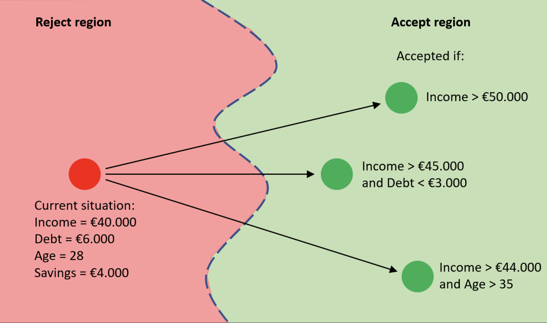 Figure 4.1: A rejected applicant (red) has multiple counterfactual paths across the ML model decision boundary into the accept region. Each arrow represents a different minimal change that achieves approval.
4.4.5 Plausibility
The counterfactual \(\mathbf{x}'\) should lie within the distribution of real data — not in an impossible or implausible region of feature space. A 22-year-old with 30 years of work experience is not a plausible counterfactual.
4.5 Key Algorithms
4.5.1 Wachter et al. (2017) — The Foundational Approach
The original formulation by Wachter, Mittelstadt, and Russell is gradient-based. Starting from \(\mathbf{x}\), it performs gradient descent in feature space to find \(\mathbf{x}'\) that satisfies the objective above.
Strengths: - Simple and model-agnostic (via numerical gradients) - Well-studied theoretically
Limitations: - Generates a single counterfactual - Does not enforce actionability or plausibility - Can land in implausible data regions
4.5.2 DiCE — Diverse Counterfactual Explanations (Mothilal et al., 2020)
DiCE (Diverse Counterfactual Explanations) directly addresses the diversity limitation. It generates a set of counterfactuals by adding a determinantal point process (DPP) diversity term to the objective:
The second term maximizes pairwise distances among the generated counterfactuals, ensuring diversity.
How does DiCE search for counterfactuals? Rather than performing gradient descent from a single starting point like Wachter et al., DiCE initializes multiple candidate counterfactuals — either randomly sampled from the feature space, or drawn from the training data points that already have the desired target class. It then jointly optimizes all \(k\) candidates simultaneously using the objective above. This means the candidates are nudged both toward the desired class (via the prediction loss term) and away from each other (via the diversity term). In practice, DiCE supports multiple backends: - Gradient-based: Uses automatic differentiation (PyTorch/TensorFlow) to directly optimize the objective for differentiable models. - KD-tree / random sampling: For black-box models, DiCE can sample counterfactuals from a k-d tree built over training data with the target class, filtering by constraints. - Genetic algorithms: An evolutionary search method that works when gradients are unavailable.
DiCE also supports: - Feature constraints: Lock immutable features (e.g., age, gender) - Range constraints: Specify allowed value ranges per feature - Proximity loss: Control how close counterfactuals are to the original
4.5.3 FACE — Feasible and Actionable Counterfactual Explanations (Poyiadzi et al., 2020)
FACE uses a graph-based approach over the training data to find counterfactuals that are not only valid but also reachable through plausible intermediate states. The key insight is that a counterfactual should not just exist in a desired region of feature space — there should be a realistic, densely-populated path that connects the original instance to it.
How it works: FACE constructs a weighted graph over the training data, where edges connect nearby data points and edge weights reflect the density of the feature space between them (e.g., using kernel density estimation). It then applies shortest-path algorithms (such as Dijkstra's) to find the path from the original instance \(\mathbf{x}\) to a target instance \(\mathbf{x}'\) that maximises traversal through high-density regions. The result is a counterfactual that is not only close in distance but feasibly reachable through the data manifold.
Think of it as the difference between: - Teleporting to the other side of a wall (Wachter) — valid destination, but no viable path - Walking through a door in the wall (FACE) — valid destination, connected by a realistic route
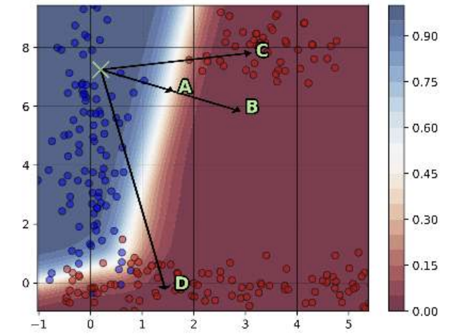
Figure 4.2: A, B, C, and D are four candidate counterfactuals of ×, where × (marked with a cross on the left) is the original instance. The x-axis and y-axis represent two input features. The background colour indicates the model's predicted probability — darker red means more confidently classified as the target class, while the light band near the decision boundary is where the model is uncertain. Blue dots are training samples from the original class; red dots are from the target class.
- A is found by minimising the ℓ₂ distance — it is the closest counterfactual, but sits in a low-density region near the boundary where real data is sparse.
- B is a generic point with a large classification margin (confidently in the target class), but it is also in a low-density area.
- C lies in a high-density region and has a large margin, but the path from × to C passes through a low-density corridor.
- D is chosen by FACE as the best counterfactual: it lies in a high-density region, has a strong classification margin, and is connected to × via a high-density path — meaning there are real, plausible data points along the way. This makes D the most feasible option: the individual can realistically transition from × to D in small, data-supported steps.
Source: Poyiadzi et al., 2020
4.5.4 Growing Spheres (Laugel et al., 2017)
This model-agnostic approach generates counterfactuals by sampling random points in expanding spheres around \(\mathbf{x}\) until a point with the desired prediction is found. Simple but effective for black-box models.
4.6 Worked Example: Loan Application
Let's make this concrete with a worked Python example using DiCE.
Setup
pip install dice-ml scikit-learn pandas
Training a Simple Classifier
import pandas as pd
from sklearn.ensemble import RandomForestClassifier
from sklearn.model_selection import train_test_split
import dice_ml

# Simulate a loan dataset
data = pd.DataFrame({
    'income': [30000, 45000, 60000, 25000, 80000, 50000, 35000, 70000],
    'loan_amount': [10000, 15000, 20000, 8000, 25000, 12000, 11000, 22000],
    'credit_score': [580, 700, 750, 550, 800, 680, 600, 720],
    'employment_years': [1, 5, 10, 0, 15, 6, 2, 8],
    'approved': [0, 1, 1, 0, 1, 1, 0, 1]
})

X = data.drop('approved', axis=1)
y = data['approved']

X_train, X_test, y_train, y_test = train_test_split(X, y, test_size=0.2, random_state=42)

model = RandomForestClassifier(n_estimators=100, random_state=42)
model.fit(X_train, y_train)
Generating Counterfactuals with DiCE
# Wrap data for DiCE
d = dice_ml.Data(
    dataframe=data,
    continuous_features=['income', 'loan_amount', 'credit_score', 'employment_years'],
    outcome_name='approved'
)

# Wrap model
m = dice_ml.Model(model=model, backend='sklearn')

# Create explanation object
exp = dice_ml.Dice(d, m, method='random')

# Query instance: applicant who was rejected
query_instance = pd.DataFrame({
    'income': [30000],
    'loan_amount': [10000],
    'credit_score': [580],
    'employment_years': [1]
})

# Generate 3 diverse counterfactuals
dice_exp = exp.generate_counterfactuals(
    query_instance,
    total_CFs=3,
    desired_class='opposite',
    features_to_vary=['income', 'credit_score', 'employment_years']  # actionable only
)

dice_exp.visualize_as_dataframe()
Sample Output
| income | loan_amount | credit_score | employment_years | approved |
|---|---|---|---|---|
| 30000 (original) | 10000 | 580 | 1 | ❌ 0 |
| 47000 | 10000 | 580 | 1 | ✅ 1 |
| 30000 | 10000 | 690 | 4 | ✅ 1 |
| 38000 | 10000 | 640 | 3 | ✅ 1 |
Three different paths to approval — the applicant can choose the most feasible one.
4.7 Contrastive Explanations: "Why This, Not That?"
While counterfactuals ask what to change, contrastive explanations compare a factual prediction against an alternative prediction directly.
The Formal Contrast
Given:
- \(\mathbf{x}\): the actual input
- \(f(\mathbf{x}) = y\): the actual prediction
- \(\mathbf{x}_{foil}\): a foil (comparison instance)
- \(f(x_{foil}) = y_{foil}\): the foil's prediction
A contrastive explanation answers: "Why did \(f(\mathbf{x}) = y\) and not \(y_{foil}\)?"
The explanation identifies which features differ between \(\mathbf{x}\) and \(\mathbf{x}_{foil}\) and how those differences drive the prediction difference.
Example
"Why was applicant A rejected but applicant B with similar income approved?"
"Because applicant A has a credit score of 580 vs. 700 for applicant B. This 120-point difference in credit score is the primary driver of the different decisions."
This is more intuitive than abstract feature importance because it grounds the explanation in a real comparison.
Connection to Shapley Values
Contrastive explanations can be linked to SHAP (Chapter 3). A SHAP explanation \(\phi_i(\mathbf{x})\) expresses the contribution of feature \(i\) relative to a background distribution. By setting the background to a specific foil \(\mathbf{x}_{foil}\), SHAP becomes a contrastive explanation:
4.8 Legal and Ethical Implications
4.8.1 The GDPR and the "Right to Explanation"
The General Data Protection Regulation (GDPR), in force since 2018 across the EU, contains Article 22, which grants individuals the right to not be subject to solely automated decision-making that significantly affects them — including a right to obtain "meaningful information about the logic involved."
Wachter et al. (2017) argue that counterfactual explanations are a practical implementation of this right. They: - Do not require revealing the model's parameters (protecting trade secrets) - Do give the individual actionable information about their decision - Are model-agnostic, so they apply to any automated system
This makes counterfactuals particularly well-suited to regulated domains: credit scoring, hiring, insurance, and criminal risk assessment.
4.8.2 Algorithmic Recourse
Algorithmic recourse (Ustun et al., 2019) is the right of an individual to contest and change an algorithmic decision through personal action. It is not enough to explain a decision — a fair system should provide a feasible path to a different outcome.
This raises a deeper question: is it ethical to give a counterfactual that is technically valid but practically impossible? Consider:
"If you had graduated from university, you would have been hired."
This is a valid counterfactual but provides no actionable recourse to someone who cannot go back in time and change their education. Good recourse must account for:
- Causal constraints: You cannot change your age; increasing income may require changing job — which affects other features causally.
- Cost: Some changes are expensive or time-consuming.
- Uncertainty: The model may change over time; a counterfactual valid today may not be valid next year.
4.8.3 Fairness Concerns
Counterfactuals can inadvertently encode bias. If the training data reflects historical discrimination:
- The model may require minority applicants to clear higher bars for approval
- Counterfactuals will reflect this: a minority applicant's counterfactual may require a higher income than a majority applicant's
Algorithmic fairness research (see Chapter 10) connects deeply here. Counterfactual fairness (Kusner et al., 2017) defines a decision as fair if it would remain the same in a counterfactual world where a protected attribute (race, gender) had been different — keeping all causally downstream features fixed.
4.9 Evaluation of Counterfactual Methods
How do we evaluate whether a counterfactual explanation system is good? Key metrics include:
| Metric | Description |
|---|---|
| Validity | Does the CF actually flip the prediction? |
| Proximity | How close (in distance) is CF to original? |
| Sparsity | How many features changed? |
| Diversity | How different are multiple CFs from each other? |
| Plausibility | Does CF lie in a high-density region of data? |
| Actionability | Are all changed features actionable? |
No single algorithm excels on all metrics. There is an inherent tension: - Proximity vs. Plausibility: The closest point across the decision boundary may be implausible - Diversity vs. Proximity: Diverse CFs are by definition more spread out, so some will be farther away - Sparsity vs. Validity: Changing fewer features may make it harder to find a valid CF
4.10 Reflective Questions
Before moving to the next chapter, consider:
-
A hiring algorithm rejects a candidate. The counterfactual says: "If you had 3 more years of experience, you would have been hired." Is this a good explanation? Is it fair? Is it actionable?
-
How does a counterfactual differ from a nearest neighbor in the training data? When would these coincide, and when would they differ?
-
GDPR's right to explanation applies to "significant" automated decisions. Should counterfactual explanations be legally mandated for all ML-driven decisions, or only some? Where would you draw the line?
-
If a bank knows customers will game their counterfactuals (e.g., temporarily inflating income), how should this affect the design of counterfactual explanation systems?
-
Counterfactuals in a recidivism risk model might say: "If you had not been arrested before age 18, your score would be lower." Critique this from a fairness and causal perspective.
4.11 Summary
This chapter introduced two closely related but distinct approaches to explaining machine learning decisions:
- Contrastive explanations answer "why P rather than Q?" — grounding explanations in comparisons between actual and alternative outcomes.
- Counterfactual explanations answer "what would need to change to get a different outcome?" — providing actionable, minimal-change paths to alternative decisions.
We saw how these concepts are rooted in cognitive science (Byrne, 2019), formally defined as optimization problems (Wachter et al., 2017), and implemented by practical tools like DiCE. We examined what makes a good counterfactual (validity, sparsity, diversity, plausibility, actionability) and explored their legal significance under GDPR and the broader concept of algorithmic recourse.
Critically, counterfactual explanations do not expose model internals — making them compatible with commercial secrecy — while still providing individuals with meaningful, actionable information about decisions that affect their lives. This balance makes them one of the most practically impactful methods in the interpretable ML toolkit.
In the next chapter, we turn to Example and Case-based Explanations, which extend this comparative logic to entire sets of training examples rather than single counterfactual instances.
References
Byrne, R. M. J. (2019). Counterfactuals in Explainable Artificial Intelligence (XAI): Evidence from Human Reasoning. Proceedings of the 28th International Joint Conference on Artificial Intelligence (IJCAI). https://doi.org/10.24963/ijcai.2019/876
Karimi, A. H., Barthe, G., Balle, B., & Valera, I. (2020). Model-Agnostic Counterfactual Explanations for Consequential Decisions. Proceedings of the 23rd International Conference on Artificial Intelligence and Statistics (AISTATS).
Kusner, M. J., Loftus, J. R., Russell, C., & Silva, R. (2017). Counterfactual Fairness. Advances in Neural Information Processing Systems (NeurIPS).
Laugel, T., Lesot, M.-J., Marsala, C., Renard, X., & Detyniecki, M. (2017). Inverse Classification for Comparison-based Interpretability in Machine Learning. arXiv:1712.08443.
Lipton, P. (1990). Contrastive Explanation. Royal Institute of Philosophy Supplements, 27, 247–266.
Mothilal, R. K., Sharma, A., & Tan, C. (2020). Explaining Machine Learning Classifiers through Diverse Counterfactual Explanations. Proceedings of the 2020 ACM FAT* Conference. https://doi.org/10.1145/3351095.3372850
Poyiadzi, R., Sokol, K., Santos-Rodriguez, R., De Bie, T., & Flach, P. (2020). FACE: Feasible and Actionable Counterfactual Explanations. Proceedings of the AAAI/ACM Conference on AI, Ethics, and Society.
Ustun, B., Spangher, A., & Liu, Y. (2019). Actionable Recourse in Linear Classification. Proceedings of the ACM FAT* Conference. https://doi.org/10.1145/3287560.3287566
Wachter, S., Mittelstadt, B., & Russell, C. (2017). Counterfactual Explanations without Opening the Black Box: Automated Decisions and the GDPR. Harvard Journal of Law & Technology, 31(2). https://doi.org/10.2139/ssrn.3063289
Citation
If you found this chapter useful, please cite it as:
@misc{amr_2026_XAI,
  author       = {Youssef Amr},
  title        = {Interpreting Machine Learning: A Gentle Introduction, Chapter 4},
  year         = {2026},
  publisher    = {GitHub},
  howpublished = {\url{https://github.com/amrmsab/interpreting_machine_learning}},
}